Theory of CSEP Tests
This page describes the theory of each of the forecast tests included in pyCSEP along with working code examples. You will find information on the goals of each test, the theory behind the tests, how the tests are applied in practice, and how forecasts are ‘scored’ given the test results. Also, we include the code required to run in each test and a description of how to interpret the test results.
import csep
from csep.core import (
    regions,
    catalog_evaluations,
    poisson_evaluations as poisson
)
from csep.utils import (
    datasets,
    time_utils,
    comcat,
    plots,
    readers
)

# Filters matplotlib warnings
import warnings
warnings.filterwarnings('ignore')
Grid-based Forecast Tests
These tests are designed for grid-based forecasts (e.g., Schorlemmer et al., 2007), where expected rates are provided in discrete Poisson space-magnitude cells covering the region of interest. The region \(\boldsymbol{R}\) is then the product of the spatial rate \(\boldsymbol{S}\) and the binned magnitude rate \(\boldsymbol{M}\),
A forecast \(\boldsymbol{\Lambda}\) can be fully specified as the expected number of events (or rate) in each space-magnitude bin (\(m_i, s_j\)) covering the region \(\boldsymbol{R}\) and therefore can be written as
where \(\lambda_{m_i, s_j}\) is the expected rate of events in magnitude bin \(m_i\) and spatial bin \(s_j\). The observed catalogue of events \(\boldsymbol{\Omega}\) we use to evaluate the forecast is similarly discretised into the same space-magnitude bins, and can be described as
where \(\omega_{m_i, s_j}\) is the observed number of events in spatial cell \(s_j\) and magnitude bin \(m_i\). The magnitude bins are specified in the forecast: typically these are in 0.1 increments and this is the case in the examples we use here. These examples use the Helmstetter et al (2007) smoothed seismicity forecast (including aftershocks), testing over a 5 year period between 2010 and 2015.
# Set up experiment parameters
start_date = time_utils.strptime_to_utc_datetime('2010-01-01 00:00:00.0')
end_date = time_utils.strptime_to_utc_datetime('2015-01-01 00:00:00.0')

# Loads from the PyCSEP package
helmstetter = csep.load_gridded_forecast(
    datasets.helmstetter_aftershock_fname,
    start_date=start_date,
    end_date=end_date,
    name='helmstetter_aftershock'
)

# Set up evaluation catalog
catalog = csep.query_comcat(helmstetter.start_time, helmstetter.end_time,
                            min_magnitude=helmstetter.min_magnitude)

# Filter evaluation catalog
catalog = catalog.filter_spatial(helmstetter.region)

# Add seed for reproducibility in simulations
seed = 123456

# Number of simulations for Poisson consistency tests
nsim = 100000
Fetched ComCat catalog in 5.9399449825286865 seconds.

Downloaded catalog from ComCat with following parameters
Start Date: 2010-01-10 00:27:39.320000+00:00
End Date: 2014-08-24 10:20:44.070000+00:00
Min Latitude: 31.9788333 and Max Latitude: 41.1431667
Min Longitude: -125.3308333 and Max Longitude: -115.0481667
Min Magnitude: 4.96
Found 24 events in the ComCat catalog.
Consistency tests
The consistency tests evaluate the consistency of a forecast against observed earthquakes. These tests were developed across a range of experiments and publications (Schorlemmer et al, 2007; Zechar et al 2010; Werner et al, 2011a). The consistency tests are based on the likelihood of observing the catalogue (actual recorded events) given the forecast. Since the space-magnitude bins are assumed to be independent, the joint-likelihood of observing the events in each individual bin given the specified forecast can be written as
where \(f_{m_i, s_j}\) specifies the probability distribution in each space-magnitude bin. We prefer to use the joint log-likelihood in order to sum log-likelihoods rather than multiply the likelihoods. The joint log-likelihood can be written as:
The likelihood of the observations, \(\boldsymbol{\Omega}\), given the forecast \(\boldsymbol{\Lambda}\) is the sum over all space-magnitude bins of the log probabilities in individual cells of the forecast. Grid-based forecasts are specified by the expected number of events in a discrete space-magnitude bin. From the maximum entropy principle, we assign a Poisson distribution in each bin. In this case, the probability of an event occurring is independent of the time since the last event, and events occur at a rate \(\lambda\). The Poissonian joint log-likelihood can be written as
where \(\lambda(m_i, s_j)\) and \(\omega(m_i, s_j)\) are the expected counts from the forecast and observed counts in cell \(m_i, s_j\) respectively. We can calculate the likelihood directly given the forecast and discretised observations.
Forecast uncertainty
A simulation based approach is used to account for uncertainty in the forecast. We simulate realizations of catalogs that are consistent with the forecast to obtain distributions of scores. In the pyCSEP package, as in the original CSEP tests, simulation is carried out using the cumulative probability density of the forecast obtained by ordering the rates in each bin. We shall call \(F_{m_is_j}\) the cumulative probability density in cell \((m_i, s_j)\). The simulation approach then works as follows:
For each forecast bin, draw a random number \(z\) from a uniform distribution between 0 and 1
Assign this event to a space-magnitude bin through the inverse cumulative density distribution at this point \(F^{-1}_{m_i, s_j}(z)\)
Iterate over all simulated events to generate a catalog containing \(N_{sim}\) events consistent with the forecast
For each of these tests, we can plot the distribution of likelihoods
computed from theses simulated catalogs relative to the observations
using the plots.plot_poisson_consistency_test function. We also
calculate a quantile score to diagnose a particular forecast with
repsect. The number of simulations can be supplied to the Poisson
consistency test functions using the num_simulations argument: for
best results we suggest 100,000 simulations to ensure convergence.
Scoring the tests
Through simulation (as described above), we obtain a set of simulated catalogs \(\{\hat{\boldsymbol{\Omega}}\}\). Each catalogue can be written as
where \(\hat{\lambda}_x(m_i, s_j)\) is the number of simulated earthquakes in cell \((m_i, s_j)\) of (simulated) catalog \(x\) that is consistent with the forecast \(\Lambda\). We then compute the joint log-likelihood for each simulated catalogue \(\hat{L}_x = L(\hat{\Omega}_x|\Lambda)\). The joint log-likelihood for each simulated catalogue given the forecast gives us a set of log-likelihoods \(\{\hat{\boldsymbol{L}}\}\) that represents the range of log-likelihoods consistent with the forecast. We then compare our simulated log-likelihoods with the observed log-likelihood \(L_{obs} = L(\boldsymbol{\Omega}|\boldsymbol{\Lambda})\) using a quantile score.
The quantile score is defined by the fraction of simulated joint log-likelihoods less than or equal to the observed likelihood.
Whether a forecast can be said to pass an evaluation depends on the significance level chosen for the testing process. The quantile score explicitly tells us something about the significance of the result: the observation is consistent with the forecast with \(100(1-\gamma)\%\) confidence (Zechar, 2011). Low \(\gamma\) values demonstrate that the observed likelihood score is less than most of the simulated catalogs. The consistency tests, excluding the N-test, are considered to be one-sided tests: values which are too small are ruled inconsistent with the forecast, but very large values may not necessarily be inconsistent with the forecast and additional testing should be used to further clarify this (Schorlemmer et al, 2007).
Different CSEP experiments have used different sensitivity values. Schorlemmer et al (2010b) consider \(\gamma \lt 0.05\) while the implementation in the Italian CSEP testing experiment uses \(\gamma\) < 0.01 (Taroni et al, 2018). However, the consistency tests are most useful as diagnostic tools where the quantile score assesses the level of consistency between observations and data. Temporal variations in seismicity make it difficult to formally reject a model from a consistency test over a single evaluation period.
Likelihood-test (L-test)
Aim: Evaluate the likelihood of observed events given the provided forecast - this includes the rate, spatial distribution and magnitude components of the forecast.
Method: The L-test is one of the original forecast tests described in Schorlemmer et al, 2007. The likelihood of the observation given the model is described by a Poisson likelihood function in each cell and the total joint likelihood described by the product over all bins, or the sum of the log-likelihoods (see above, or Zechar 2011 for more details).
Note: The likelihood scores are dominated by the rate-component of the forecast. This causes issues in scoring forecasts where the expected number of events are different from the observed number of events. We suggest to use the N-test (below) and CL-test (below) independently to score the rate component, and spatial-magnitude components of the forecast. This behavior can be observed by comparing the CL-test and N-test results with the L-test results in this notebook. Since the forecast overpredicts the rate of events during this testing period, the L-test provides a passing score even though the space-magnitude and rate components perform poorly during this evaluation period.
pyCSEP implementation
pyCSEP uses the forecast and catalog and returns the test distribution,
observed statistic and quantile score, which can be accessed from the
likelihood_test_result object. We can pass this directly to the
plotting function, specifying that the test should be one-sided.
likelihood_test_result = poisson.likelihood_test(
    helmstetter,
    catalog,
    seed=seed,
    num_simulations=nsim
)
ax = plots.plot_poisson_consistency_test(
    likelihood_test_result,
    one_sided_lower=True,
    plot_args={'title': r'$\mathcal{L}-\mathrm{test}$', 'xlabel': 'Log-likelihood'}
)
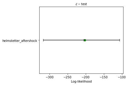
pyCSEP plots the resulting \(95\%\) range of likelihoods returned by the simulation with the black bar by default. The observed likelihood score is shown by a green square where the forecast passes the test and a red circle where the observed likelihood is outside the likelihood distribution.
CL-test
Aim: The original likelihood test described above gives a result that combines the spatial, magnitude and number components of a forecast. The conditional likelihood or CL-Test was developed to test the spatial and magnitude performance of a forecast without the influence of the number of events (Werner et al. 2011a, 2011b). By conditioning the test distribution on the observed number of events we elimiate the dependency with the forecasted number of events as described above.
Implementation in pyCSEP
cond_likelihood_test_result = poisson.conditional_likelihood_test(
    helmstetter,
    catalog,
    seed=seed,
    num_simulations=nsim
)
ax = plots.plot_poisson_consistency_test(
    cond_likelihood_test_result,
    one_sided_lower=True,
    plot_args = {'title': r'$CL-\mathrm{test}$', 'xlabel': 'conditional log-likelihood'}
)
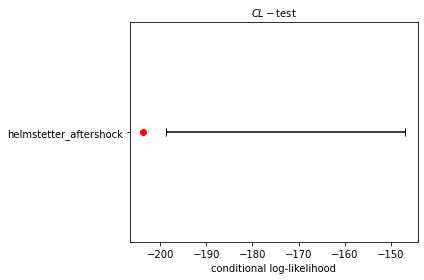
Again, the \(95\%\) confidence range of likelihoods is shown by the black bar, and the symbol reflects the observed conditional-likelihood score. In this case, the observed conditional-likelihood is shown with the red circle, which falls outside the range of likelihoods simulated from the forecast. To understand why the L- and CL-tests give different results, consider the results of the N-test and S-test in the following sections.
N-test
Aim: The number or N-test is the most conceptually simple test of a forecast: To test whether the number of observed events is consistent with that of the forecast.
Method: The originial N-test was introduced by Schorlemmer et al (2007) and modified by Zechar et al (2010). The observed number of events is given by,
Using the simulations described above, the expected number of events is calculated by summing the simulated number of events over all grid cells
where \(\hat{\omega}_x(m_i, s_j)\) is the simulated number of events in catalog \(x\) in spatial cell \(s_j\) and magnitude cell \(m_i\), generating a set of simulated rates \(\{ \hat{N} \}\). We can then calculate the probability of i) observing at most \(N_{obs}\) events and ii) of observing at least \(N_{obs}\) events. These probabilities can be written as:
and
If a forecast is Poisson, the expected number of events in the forecast follows a Poisson distribution with expectation \(N_{fore} = \sum_{m_i, s_j \in R} \lambda(m_i, s_j)\). The cumulative distribution is then a Poisson cumulative distribution:
which can be used directly without the need for simulations. The N-test quantile score is then
and
The original N-test considered only \(\delta_2\) and it’s complement \(1-\delta_2\), which effectively tested the probability of at most \(N_{obs}\) events and more than \(N_{obs}\) events. Very small or very large values (<0.025 or > 0.975 respectively) were considered to be inconsistent with the forecast in Schorlemmer et al (2010). However the approach above aims to test something subtely different, that is at least \(N_{obs}\) events and at most \(N_{obs}\) events. Zechar et al (2010a) recommends testing both \(\delta_1\) and \(\delta_2\) with an effective significance of have the required significance level, so for a required significance level of 0.05, a forecast is consistent if both \(\delta_1\) and \(\delta_2\) are greater than 0.025. A very small \(\delta_1\) suggest the rate is too low while a very low \(\delta_2\) suggests a rate which is too high to be consistent with observations.
Implementation in pyCSEP
pyCSEP uses the Zechar et al (2010) version of the N-test and the
cumulative Poisson approach to estimate the range of expected events
from the forecasts, so does not implement a simulation in this case. The
upper and lower bounds for the test are determined from the cumulative
Poisson distribution. number_test_result.quantile will return both
\(\delta_1\) and \(\delta_2\) values.
number_test_result = poisson.number_test(helmstetter, catalog)
ax = plots.plot_poisson_consistency_test(
    number_test_result,
    plot_args={'xlabel':'Number of events'}
)
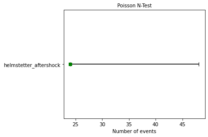
In this case, the black bar shows the \(95\%\) interval for the number of events in the forecast. The actual observed number of events is shown by the green box, which just passes the N-test in this case: the forecast generallly expects more events than are observed in practice, but the observed number falls just within the lower limits of what is expected so the forecast (just!) passes the N-test.
M-test
Aim: Establish consistency (or lack thereof) of observed event magnitudes with forecast magnitudes.
Method: The M-test is first described in Zechar et al. (2010) and aims to isolate the magnitude component of a forecast. To do this, we sum over the spatial bins and normalise so that the sum of events matches the observations.
where
and
where
Then we compute the joint log-likelihood as we did for the L-test:
We then wish to compare this with the distribution of simulated log-likelihoods, this time keep the number of events fixed to
\(N_{obs}\). Then for each simulated catalogue, \(\hat{M}_x = L(\hat{\boldsymbol{\Omega}}^m | \boldsymbol{\Lambda}^m)\)
Quantile score: The final test statistic is again the fraction of observed log likelihoods within the range of the simulated log likelihood values:
and the observed magnitudes are inconsistent with the forecast if \(\kappa\) is less than the significance level.
pyCSEP implementation
mag_test_result = poisson.magnitude_test(
    helmstetter,
    catalog,
    seed=seed,
    num_simulations=nsim
)
ax = plots.plot_poisson_consistency_test(
    mag_test_result,
    one_sided_lower=True,
    plot_args={'xlabel':'Normalized likelihood'}
)
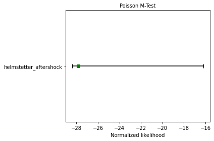
In this example, the forecast passes the M-test, demonstrating that the magnitude distribution in the forecast is consistent with observed events. This is shown by the green square marking the joint log-likelihood for the observed events.
S-test
Aim: The spatial or S-test aims to establish consistency (or lack thereof) of observed event locations with a forecast. It is originally defined in Zechar et al (2010).
Method: Similar to the M-test, but in this case we sum over all magnitude bins.
where
and
where
Then we compute the joint log-likelihood as we did for the L-test or the M-test:
We then wish to compare this with the distribution of simulated log-likelihoods, this time keeping the number of events fixed to \(N_{obs}\). Then for each simulated catalogue, \(\hat{S}_x = L(\hat{\boldsymbol{\Omega}}^s | \boldsymbol{\Lambda}^s)\)
The final test statistic is again the fraction of observed log likelihoods within the range of the simulated log likelihood values:
and again the distinction between a forecast passing or failing the test depends on our significance level.
pyCSEP implementation
The S-test is again a one-sided test, so we specify this when plotting the result.
spatial_test_result = poisson.spatial_test(
    helmstetter,
    catalog,
    seed=seed,
    num_simulations=nsim
)
ax = plots.plot_poisson_consistency_test(
    spatial_test_result,
    one_sided_lower=True,
    plot_args = {'xlabel':'normalized spatial likelihood'}
)
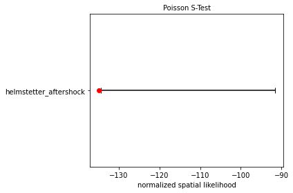
The Helmstetter model fails the S-test as the observed spatial likelihood falls in the tail of the simulated likelihood distribution. Again this is shown by a coloured symbol which highlights whether the forecast model passes or fails the test.
Forecast comparison tests
The consistency tests above check whether a forecast is consistent with observations, but do not provide a straightforward way to compare two different forecasts. A few suggestions for this focus on the information gain of one forecast relative to another (Harte and Vere-Jones 2005, Imoto and Hurukawa, 2006, Imoto and Rhoades, 2010, Rhoades et al 2011). The T-test and W-test implementations for earthquake forecast comparison are first described in Rhoades et al. (2011).
The information gain per earthquake (IGPE) of model A compared to model B is defined by \(I_{N}(A, B) = R/N\) where R is the rate-corrected log-likelihood ratio of models A and B gven by
If we set \(X_i=\log\lambda_A(k_i)\) and \(Y_i=\log\lambda_B(k_i)\) then we can define the information gain per earthquake (IGPE) as
If \(I(A, B)\) differs significantly from 0, the model with the lower likelihood can be rejected in favour of the other.
t-test
If \(X_i - Y_i\) are independent and come from the same normal population with mean \(\mu\) then we can use the classic paired t-test to evaluate the null hypothesis that \(\mu = (\hat{N}_A - \hat{N}_B)/N\) against the alternative hypothesis \(\mu \ne (\hat{N}_A - \hat{N}_B)/N\). To implement this, we let \(s\) denote the sample variance of \((X_i - Y_i)\) such that
Under the null hypothesis \(T = I_N(A, B)\big{/}\big{(}s/\sqrt{N}\big{)}\) has a t-distribution with \(N-1\) degrees of freedom and the null hypothesis can be rejected if \(|T|\) exceeds a critical value of the \(t_{N-1}\) distribution. The confidence intervals for \(\mu - (\hat{N}_A - \hat{N}_B)/N\) can then be constructed with the form \(I_N(A,B) \pm ts/\sqrt{N}\) where t is the appropriate quantile of the \(t_{N-1}\) distribution.
W-test
An alternative to the t-test is the Wilcoxan signed-rank test or W-test. This is a non-parameteric alternative to the t-test which can be used if we do not feel the assumption of normally distributed differences in \(X_i - Y_i\) is valid. This assumption might b particularly poor when we have small sample sizes. The W-test instead depends on the (weaker) assumption that \(X_i - Y_i\) is symmetric and tests whether the meadian of \(X_i - Y_i\) is equal to \((\hat{N}_A - \hat{N}_B)/N\). The W-test is less powerful than the T-test for normally distributed differences and cannot reject the null hypothesis (with \(95\%\) confidence) for very small sample sizes (\(N \leq 5\)).
The t-test becomes more accurate as \(N \rightarrow \infty\) due to the central limit theorem and therefore the t-test is considered dependable for large \(N\). Where \(N\) is small, a model might only be considered more informative if both the t- and W-test results agree.
Implementation in pyCSEP
The t-test and W-tests are implemented in pyCSEP as below.
helmstetter_ms = csep.load_gridded_forecast(
    datasets.helmstetter_mainshock_fname,
    name = "Helmstetter Mainshock"
)

t_test = poisson.paired_t_test(helmstetter, helmstetter_ms, catalog)
w_test = poisson.w_test(helmstetter, helmstetter_ms, catalog)
comp_args = {'title': 'Paired T-test Result',
             'ylabel': 'Information gain',
             'xlabel': '',
             'xticklabels_rotation': 0,
             'figsize': (6,4)}

ax = plots.plot_comparison_test([t_test], [w_test], plot_args=comp_args)
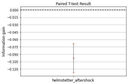
The first argument to the paired_t_test function is taken as model A
and the second as our basline model, or model B. When plotting the
result, the horizontal dashed line indicates the performance of model B
and the vertical bar shows the confidence bars for the information gain
\(I_N(A, B)\) associated with model A relative to model B. In this
case, the model with aftershocks performs statistically worse than the
benchmark model. We note that this comparison is used for demonstation
purposes only.
Catalog-based forecast tests
Catalog-based forecast tests evaluate forecasts using simulated outputs in the form of synthetic earthquake catalogs. Thus, removing the need for the Poisson approximation and simulation procedure used with grid-based forecasts. We know that observed seismicity is overdispersed with respect to a Poissonian model due to spatio-temporal clustering. Overdispersed models are more likely to be rejected by the original Poisson-based CSEP tests (Werner et al, 2011a). This modification of the testing framework allows for a broader range of forecast models. The distribution of realizations is then compared with observations, similar to in the grid-based case. These tests were developed by Savran et al 2020, who applied them to test forecasts following the 2019 Ridgecrest earthquake in Southern California.
In the following text, we show how catalog-based forecasts are defined. Again we begin by defining a region \(\boldsymbol{R}\) as a function of some magnitude range \(\boldsymbol{M}\), spatial domain \(\boldsymbol{S}\) and time period \(\boldsymbol{T}\)
An earthquake \(e\) can be described by a magnitude \(m_i\) at some location \(s_j\) and time \(t_k\). A catalog is simply a collection of earthquakes, thus the observed catalog can be written as
and a forecast is then specified as a collection of synthetic catalogs containing events \(\hat{e}_{nj}\) in domain \(\boldsymbol{R}\), as
That is, a forecast consists of \(J\) simulated catalogs each containing \(N_j\) events, described in time, space and magnitude such that \(\hat{e}_{nj}\) describes the \(n\)th synthetic event in the \(j\)th synthetic catalog \(\Lambda_j\)
When using simulated forecasts in pyCSEP, we must first explicitly specify the forecast region by specifying the spatial domain and magnitude regions as below. In effect, these are filters applied to the forecast and observations to retain only the events in \(\boldsymbol{R}\). The examples in this section are catalog-based forecast simulations for the Landers earthquake and aftershock sequence generated using UCERF3-ETAS (Field et al, 2017).
# Define the start and end times of the forecasts
start_time = time_utils.strptime_to_utc_datetime("1992-06-28 11:57:35.0")
end_time = time_utils.strptime_to_utc_datetime("1992-07-28 11:57:35.0")

# Magnitude bins properties
min_mw = 4.95
max_mw = 8.95
dmw = 0.1

# Create space and magnitude regions.
magnitudes = regions.magnitude_bins(min_mw, max_mw, dmw)
region = regions.california_relm_region()
space_magnitude_region = regions.create_space_magnitude_region(
    region,
    magnitudes
)

# Load forecast
forecast = csep.load_catalog_forecast(
    datasets.ucerf3_ascii_format_landers_fname,
    start_time = start_time,
    end_time = end_time,
    region = space_magnitude_region,
    apply_filters = True
)

# Compute expected rates
forecast.filters = [
    f'origin_time >= {forecast.start_epoch}',
    f'origin_time < {forecast.end_epoch}'
]
_ = forecast.get_expected_rates(verbose=False)

# Obtain Comcat catalog and filter to region
comcat_catalog = csep.query_comcat(
    start_time,
    end_time,
    min_magnitude=forecast.min_magnitude
)

# Filter observed catalog using the same region as the forecast
comcat_catalog = comcat_catalog.filter_spatial(forecast.region)
Fetched ComCat catalog in 0.31937098503112793 seconds.

Downloaded catalog from ComCat with following parameters
Start Date: 1992-06-28 12:00:45+00:00
End Date: 1992-07-24 18:14:36.250000+00:00
Min Latitude: 33.901 and Max Latitude: 36.705
Min Longitude: -118.067 and Max Longitude: -116.285
Min Magnitude: 4.95
Found 19 events in the ComCat catalog.
Number Test
Aim: As above, the number test aims to evaluate if the number of observed events is consistent with the forecast.
Method: The observed statistic in this case is given by \(N_{obs} = |\Omega|\), which is simply the number of events in the observed catalog. To build the test distribution from the forecast, we simply count the number of events in each simulated catalog.
As in the gridded test above, we can then evaluate the probabilities of at least and at most N events, in this case using the empirical cumlative distribution function of \(F_N\):
and
Implementation in pyCSEP
number_test_result = catalog_evaluations.number_test(
    forecast,
    comcat_catalog,
    verbose=False
)
ax = number_test_result.plot()
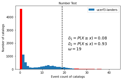
Plotting the number test result of a simulated catalog forecast displays a histogram of the numbers of events \(\hat{N}_j\) in each simulated catalog \(j\), which makes up the test distribution. The test statistic is shown by the dashed line - in this case it is the number of observed events in the catalog \(N_{obs}\).
Magnitude Test
Aim: The magnitude test aims to test the consistency of the observed frequency-magnitude distribution with that in the simulated catalogs that make up the forecast.
Method: The catalog-based magnitude test is implemented quite differently to the grid-based equivalent. We first define the union catalog \(\Lambda_U\) as the union of all simulated catalogs in the forecast. Formally:
The histograms are normalized so that the total number of events across all bins is equal to the observed number. The observed statistic is then calculated as the sum of squared logarithmic residuals between the normalised observed magnitudes and the union histograms. This statistic is related to the Kramer von-Mises statistic.
where \(\Lambda_U^{(m)}(k)\) and \(\Omega^{(m)}(k)\) represent the count in the \(k\)th bin of the magnitude-frequency distribution in the union and observed catalogs respectively. We add unity to each bin to avoid \(\log(0)\). We then build the test distribution from the catalogs in \(\boldsymbol{\Lambda}\):
where \(\lambda_j^{(m)}(k)\) represents the count in the \(k\)th bin of the magnitude-frequency distribution of the \(j\)th catalog.
The quantile score can then be calculated using the empirical CDF such that
magnitude_test_result = catalog_evaluations.magnitude_test(
    forecast,
    comcat_catalog,verbose=False
)
ax = magnitude_test_result.plot(plot_args={'xy': (0.6,0.7)})
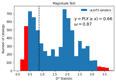
The histogram shows the resulting test distribution with \(D^*\) calculated for each simulated catalog as described in the method above. The test statistic \(\omega = d_{obs}\) is shown with the dashed horizontal line. The quantile score for this forecast is \(\gamma = 0.66\).
Pseudo-likelihood test
Aim : The pseudo-likelihood test aims to evaluate the likelihood of a forecast given an observed catalog.
Method : The pseudo-likelihood test has similar aims to the grid-based likelihood test above, but its implementation differs in a few significant ways. Firstly, it does not compute an actual likelihood (hence the name pseudo-likelihood), and instead of aggregating over cells as in the grid-based case, the pseudo-likelihood test aggregates likelihood over target event likelihood scores (so likelihood score per target event, rather than likelihood score per grid cell). The most important difference, however, is that the pseudo-likelihood tests do not use a Poisson likelihood.
The pseudo-likelihood approach is based on the continuous point process likelihood function. A continuous marked space-time point process can be specified by a conditional intensity function \(\lambda(\boldsymbol{e}|H_t)\), in which \(H_t\) describes the history of the process in time. The log-likelihood function for any point process in \(\boldsymbol{R}\) is given by
Not all models will have an explicit likelihood function, so instead we approximate the expectation of \(\lambda(e|H_t)\) using the forecast catalogs. The approximate rate density is defined as the conditional expectation given a discretised region \(R_d\) of the continuous rate
We still regard the model as continuous, but the rate density is approximated within a single cell. This is analogous to the gridded approach where we count the number of events in discrete cells. The pseudo-loglikelihood is then
and we can write the approximate rate density as
where we take the sum over all magnitude bins \(M\). We can calculate observed pseudolikelihood as
where \(\hat{\lambda}_s(k_i)\) is the approximate rate density in the \(k\)th spatial cell and \(k_i\) denotes the spatil cell in which the \(i\)th event occurs. \(\bar{N}\) is the expected number of events in \(R_d\). Similarly, we calculate the test distribution as
where \(\hat{\lambda}_s(k_{ij})\) describes the approximate rate density of the \(i\)th event in the \(j\)th catalog. We can then calculate the quantile score as
Implementation in pyCSEP
pseudolikelihood_test_result = catalog_evaluations.pseudolikelihood_test(
    forecast,
    comcat_catalog,
    verbose=False
)
ax = pseudolikelihood_test_result.plot()
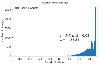
The histogram shows the test distribution of pseudolikelihood as calculated above for each catalog \(j\). The dashed vertical line shows the observed statistic \(\hat{L}_{obs} = \omega\). It is clear that the observed statistic falls within the critical region of test distribution, as reflected in the quantile score of \(\gamma_L = 0.02\).
Spatial test
Aim: The spatial test again aims to isolate the spatial component of the forecast and test the consistency of spatial rates with observed events.
Method: We perform the spatial test in the catalog-based approach in a similar way to the grid-based spatial test approach: by normalising the approximate rate density. In this case, we use the normalisation \(\hat{\lambda}_s = \hat{\lambda}_s \big/ \sum_{R} \hat{\lambda}_s\). Then the observed spatial test statistic is calculated as
in which \(\hat{\lambda}_s^*(k_i)\) is the normalised approximate rate density in the \(k\)th cell corresponding to the \(i\)th event in the observed catalog \(\Omega\). Similarly, we define the test distribution using
for each catalog j. Finally, the quantile score for the spatial test is determined by once again comparing the observed and test distribution statistics:
Implementation in pyCSEP
spatial_test_result = catalog_evaluations.spatial_test(
    forecast,
    comcat_catalog,
    verbose=False
)
ax = spatial_test_result.plot()
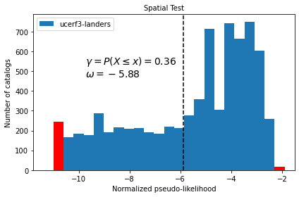
The histogram shows the test distribution of normalised pseduo-likelihood computed for each simulated catalog \(j\). The dashed vertical line shows the observed test statistic \(s_{obs} = \omega = -5.88\), which is clearly within the test distribution. The quantile score \(\gamma_s = 0.36\) is also printed on the figure by default.
Resampled Magnitude Test
Aim: Perform the resampled magnitude test for catalog-based forecasts (Serafini et al., , in-prep), which is a correction to the original M-test implementation that is biased to the total N of events.
Method: Calculates the (pseudo log-likelihood) test statistic distribution \(D_j\) from the resampled forecast’s synthetic catalogs \(\hat{\Lambda}_j\) as:
where \(\Lambda_U^{(m)}(k)\) and \(\Lambda_U^{(m)}(k)\) represent the count in the \(k\)th bin of the magnitude-frequency distribution in the union catalog and resampled catalog, respectively. The resampled catalogs \(\hat{\Lambda}_j^{(m)}\) are built from drawing exactly \(N_{obs}\) events from the union catalog \(\Lambda_U^{(m)}\).
The observed statistic is built identically as the original Magnitude test:
where \(\Omega^{(m)}(k)\) represent the count in the \(k\)th bin of the magnitude-frequency distribution in the observed catalog.
Implementation in pyCSEP
from csep.core.catalog_evaluations import resampled_magnitude_test

resampled_m_test = resampled_magnitude_test(forecast, comcat_catalog, seed=1)
resampled_m_test.plot(show = True)
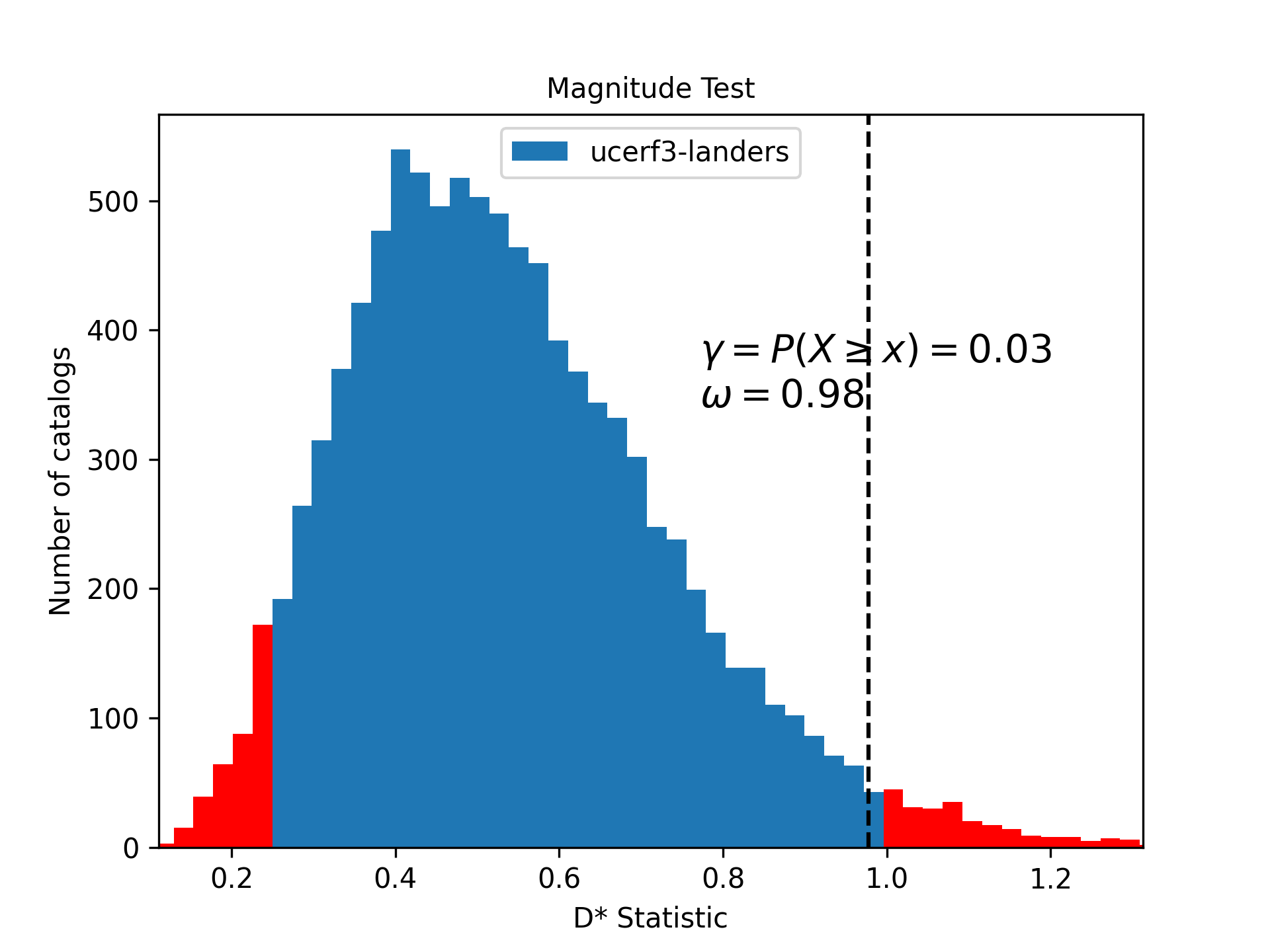
The histogram shows the resulting test distribution with \(D^*\), which has a smoother statistic distribution than the original M-test. The observed statistic \(\omega = d_{obs}\) is shown with the dashed horizontal line. The quantile score for this forecast is \(\gamma = 0.98\).
Modified Multinomial Log-Likelihood (MLL) Magnitude Test
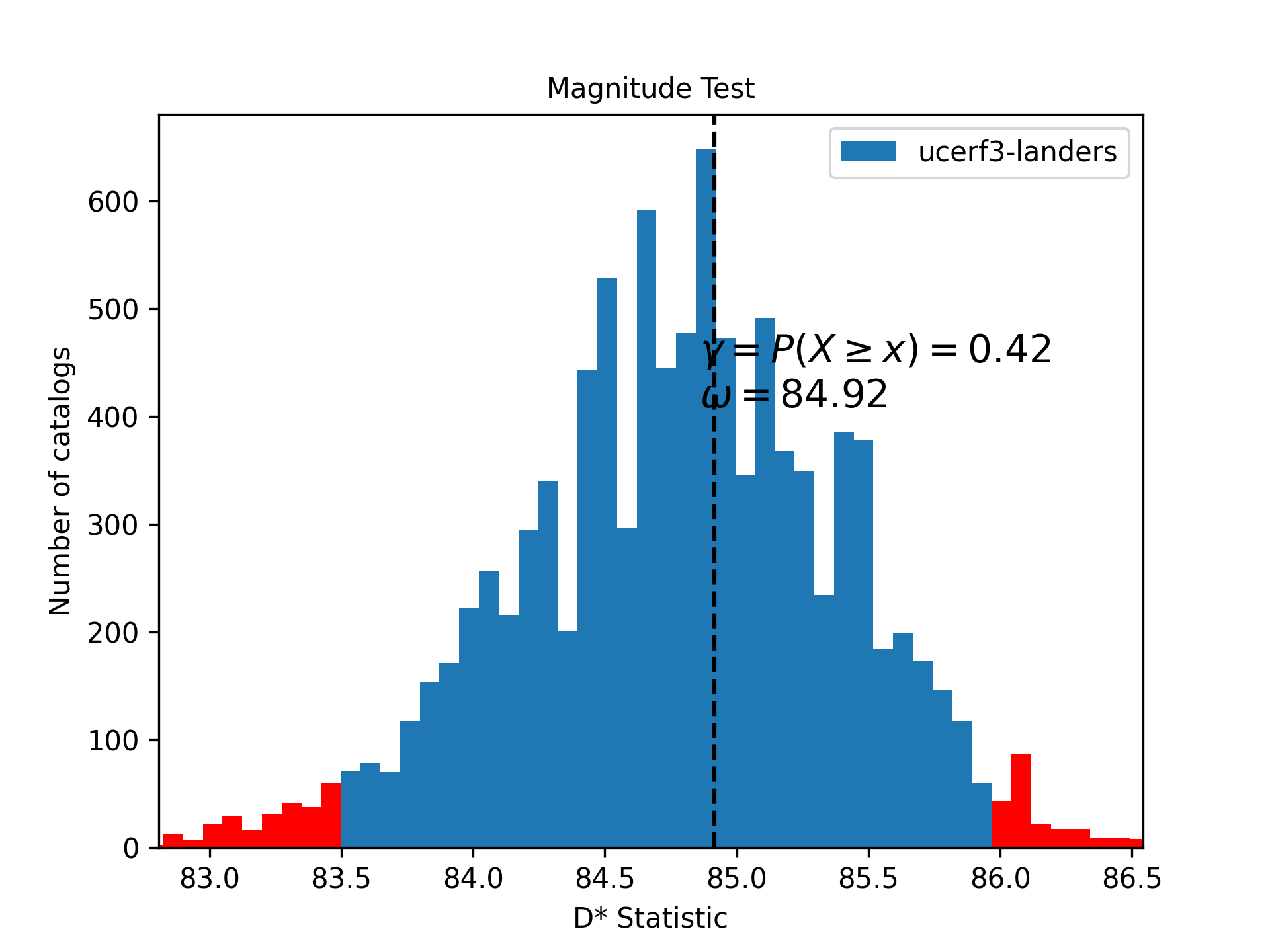
Aim: Implements the modified Multinomial log-likelihood (MLL) magnitude test (Serafini et al., in-prep).
Method: Calculates the test statistic distribution as:
\[D_j = -2 \log\Bigg[\cfrac{\mathcal{L}\big(\Lambda_u^{(m)} + \frac{N_u}{N_j}\boldsymbol{1} + \hat{\Lambda}_j^{(m)} + \boldsymbol{1}\big)} {\mathcal{L}\big(\Lambda_u^{(m)} + \frac{N_u}{N_j}\boldsymbol{1}\big) \mathcal{L}\big(\hat{\Lambda}_j^{(m)} + \boldsymbol{1}\big)}\Bigg]\]where \(\mathcal{L}\) is the multinomial likelihood function. \(\Lambda_u\) is the union of all the forecasts’ synthetic catalogs, \(\Lambda_u^{(m)}\) its magnitude histogram, and \(N_u\) the total number of events in \(\Lambda_u\). \(\hat{\Lambda}_j\) are resampled catalogs, which are built from drawing exactly \(N_{obs}\) events from the union catalog \(\Lambda_U\), whereas \(\hat{\Lambda}_j^{(m)}\) is its histogram. The vector \(\boldsymbol{1}\) has a value of 1 on each magnitude histogram bin.
The observed statistic is defined as:
\[d_{obs} = -2 \log\Bigg[\cfrac{\mathcal{L}\big(\Lambda_u^{(m)} + \frac{N_u}{N_j}\boldsymbol{1} + \Omega^{(m)} + \boldsymbol{1}\big)} {\mathcal{L}\big(\Lambda_u^{(m)} + \frac{N_u}{N_j}\boldsymbol{1}\big) \mathcal{L}\big(\Omega^{(m)} + \boldsymbol{1}\big)}\Bigg]\]The multinomial likelihood function \(\mathcal{L}\) for an arbitrary catalog’s magnitude histogram \(\Lambda^{(m)}\) is defined as:
\[\mathcal{L}(\Lambda^{(m)}) = \cfrac{N_\Lambda!}{n_{\Lambda,1}!\, ... n_{\Lambda,K}!}\prod_{k=1}^{K} \left(\cfrac{n_{\Lambda,k}}{N}\right)^{n_{\Lambda,k}}\]where \(N_\Lambda\) is the total number of events in \(\Lambda^{(m)}\), \(n_{\Lambda,k}\) the number of events in the \(k-th\) bin, and \(K\) the total number of bins.
Implementation in pyCSEP
from csep.core.catalog_evaluations import MLL_magnitude_test

MLL_t = MLL_magnitude_test(forecast, comcat_catalog, full_calculation=False, verbose=False, seed=22)
MLL_t.plot(show=True)
References
Field, E. H., K. R. Milner, J. L. Hardebeck, M. T. Page, N. J. van der Elst, T. H. Jordan, A. J. Michael, B. E. Shaw, and M. J. Werner (2017). A spatiotemporal clustering model for the third Uniform California Earthquake Rupture Forecast (UCERF3-ETAS): Toward an operational earthquake forecast, Bull. Seismol. Soc. Am. 107, 1049–1081.
Harte, D., and D. Vere-Jones (2005), The entropy score and its uses in earthquake forecasting, Pure Appl. Geophys. 162 , 6-7, 1229-1253, DOI: 10.1007/ s00024-004-2667-2.
Helmstetter, A., Y. Y. Kagan, and D. D. Jackson (2006). Comparison of short-term and time-independent earthquake forecast models for southern California, Bulletin of the Seismological Society of America 96 90-106.
Imoto, M., and N. Hurukawa (2006), Assessing potential seismic activity in Vrancea, Romania, using a stress-release model, Earth Planets Space 58 , 1511-1514.
Imoto, M., and D.A. Rhoades (2010), Seismicity models of moderate earthquakes in Kanto, Japan utilizing multiple predictive parameters, Pure Appl. Geophys. 167, 6-7, 831-843, DOI: 10.1007/s00024-010-0066-4.
Rhoades, D.A, D., Schorlemmer, M.C.Gerstenberger, A. Christophersen, J. D. Zechar & M. Imoto (2011) Efficient testing of earthquake forecasting models, Acta Geophysica 59
Savran, W., M. J. Werner, W. Marzocchi, D. Rhoades, D. D. Jackson, K. R. Milner, E. H. Field, and A. J. Michael (2020). Pseudoprospective evaluation of UCERF3-ETAS forecasts during the 2019 Ridgecrest Sequence, Bulletin of the Seismological Society of America.
Schorlemmer, D., and M.C. Gerstenberger (2007), RELM testing center, Seismol. Res. Lett. 78, 30–36.
Schorlemmer, D., M.C. Gerstenberger, S. Wiemer, D.D. Jackson, and D.A. Rhoades (2007), Earthquake likelihood model testing, Seismol. Res. Lett. 78, 17–29.
Schorlemmer, D., A. Christophersen, A. Rovida, F. Mele, M. Stucci and W. Marzocchi (2010a). Setting up an earthquake forecast experiment in Italy, Annals of Geophysics, 53, no.3
Schorlemmer, D., J.D. Zechar, M.J. Werner, E.H. Field, D.D. Jackson, and T.H. Jordan (2010b), First results of the Regional Earthquake Likelihood Models experiment, Pure Appl. Geophys., 167, 8/9, doi:10.1007/s00024-010-0081-5.
M. Taroni, W. Marzocchi, D. Schorlemmer, M. J. Werner, S. Wiemer, J. D. Zechar, L. Heiniger, F. Euchner; Prospective CSEP Evaluation of 1‐Day, 3‐Month, and 5‐Yr Earthquake Forecasts for Italy. Seismological Research Letters 2018;; 89 (4): 1251–1261. doi: https://doi.org/10.1785/0220180031
Werner, M. J., A. Helmstetter, D. D. Jackson, and Y. Y. Kagan (2011a). High-Resolution Long-Term and Short-Term Earthquake Forecasts for California, Bulletin of the Seismological Society of America 101 1630-1648
Werner, M.J. J.D. Zechar, W. Marzocchi, and S. Wiemer (2011b), Retrospective evaluation of the five-year and ten-year CSEP-Italy earthquake forecasts, Annals of Geophysics 53, no. 3, 11–30, doi:10.4401/ag-4840.
Zechar, 2011: Evaluating earthquake predictions and earthquake forecasts: a guide for students and new researchers, CORSSA (http://www.corssa.org/en/articles/theme_6/)
Zechar, J.D., M.C. Gerstenberger, and D.A. Rhoades (2010a), Likelihood-based tests for evaluating space-rate-magnitude forecasts, Bull. Seis. Soc. Am., 100(3), 1184—1195, doi:10.1785/0120090192.
Zechar, J.D., D. Schorlemmer, M. Liukis, J. Yu, F. Euchner, P.J. Maechling, and T.H. Jordan (2010b), The Collaboratory for the Study of Earthquake Predictability perspective on computational earthquake science, Concurr. Comp-Pract. E., doi:10.1002/cpe.1519.