Grid-based Forecast Evaluation

This example demonstrates how to evaluate a grid-based and time-independent forecast. Grid-based forecasts assume the variability of the forecasts is Poissonian. Therefore, Poisson-based evaluations should be used to evaluate grid-based forecasts.

Overview:

1. Define forecast properties (time horizon, spatial region, etc).

2. Obtain evaluation catalog

3. Apply Poissonian evaluations for grid-based forecasts

4. Store evaluation results using JSON format

5. Visualize evaluation results

Load required libraries

Most of the core functionality can be imported from the top-level csep package. Utilities are available from the csep.utils subpackage.

import csep
from csep.core import poisson_evaluations as poisson
from csep.utils import datasets, time_utils, plots

# Needed to show plots from the terminal
import matplotlib.pyplot as plt

Define forecast properties

We choose a Time-independent Forecast to show how to evaluate a grid-based earthquake forecast using PyCSEP. Note, the start and end date should be chosen based on the creation of the forecast. This is important for time-independent forecasts because they can be rescale to any arbitrary time period.

from csep.utils.stats import get_Kagan_I1_score

start_date = time_utils.strptime_to_utc_datetime('2006-11-12 00:00:00.0')
end_date = time_utils.strptime_to_utc_datetime('2011-11-12 00:00:00.0')

Load forecast

For this example, we provide the example forecast data set along with the main repository. The filepath is relative to the root directory of the package. You can specify any file location for your forecasts.

forecast = csep.load_gridded_forecast(datasets.helmstetter_aftershock_fname,
                                      start_date=start_date,
                                      end_date=end_date,
                                      name='helmstetter_aftershock')

Load evaluation catalog

We will download the evaluation catalog from ComCat (this step requires an internet connection). We can use the ComCat API to filter the catalog in both time and magnitude. See the catalog filtering example, for more information on how to filter the catalog in space and time manually.

print("Querying comcat catalog")
catalog = csep.query_comcat(forecast.start_time, forecast.end_time, min_magnitude=forecast.min_magnitude)
print(catalog)

Querying comcat catalog
Fetched ComCat catalog in 5.163585662841797 seconds.

Downloaded catalog from ComCat with following parameters
Start Date: 2007-02-26 12:19:54.530000+00:00
End Date: 2011-02-18 17:47:35.770000+00:00
Min Latitude: 31.9788333 and Max Latitude: 41.1444
Min Longitude: -125.0161667 and Max Longitude: -114.8398
Min Magnitude: 4.96
Found 34 events in the ComCat catalog.

        Name: None

        Start Date: 2007-02-26 12:19:54.530000+00:00
        End Date: 2011-02-18 17:47:35.770000+00:00

        Latitude: (31.9788333, 41.1444)
        Longitude: (-125.0161667, -114.8398)

        Min Mw: 4.96
        Max Mw: 7.2

        Event Count: 34

Filter evaluation catalog in space

We need to remove events in the evaluation catalog outside the valid region specified by the forecast.

catalog = catalog.filter_spatial(forecast.region)
print(catalog)

Name: None

Start Date: 2007-02-26 12:19:54.530000+00:00
End Date: 2011-02-18 17:47:35.770000+00:00

Latitude: (31.9788333, 41.1155)
Longitude: (-125.0161667, -115.0481667)

Min Mw: 4.96
Max Mw: 7.2

Event Count: 32

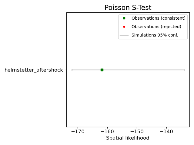
Compute Poisson spatial test

Simply call the csep.core.poisson_evaluations.spatial_test() function to evaluate the forecast using the specified evaluation catalog. The spatial test requires simulating from the Poisson forecast to provide uncertainty. The verbose option prints the status of the simulations to the standard output.

spatial_test_result = poisson.spatial_test(forecast, catalog)

Store evaluation results

PyCSEP provides easy ways of storing objects to a JSON format using csep.write_json(). The evaluations can be read back into the program for plotting using csep.load_evaluation_result().

csep.write_json(spatial_test_result, 'example_spatial_test.json')

Plot spatial test results

We provide the function csep.utils.plotting.plot_poisson_consistency_test() to visualize the evaluation results from consistency tests.

ax = plots.plot_poisson_consistency_test(spatial_test_result,
                                        plot_args={'xlabel': 'Spatial likelihood'})
plt.show()

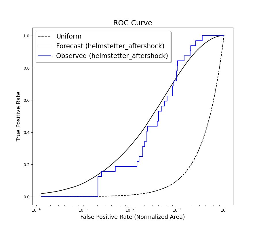
Plot ROC Curves

We can also plot the Receiver operating characteristic (ROC) Curves based on forecast and testing-catalog. In the figure below, True Positive Rate is the normalized cumulative forecast rate, after sorting cells in decreasing order of rate. The “False Positive Rate” is the normalized cumulative area. The dashed line is the ROC curve for a uniform forecast, meaning the likelihood for an earthquake to occur at any position is the same. The further the ROC curve of a forecast is to the uniform forecast, the specific the forecast is. When comparing the forecast ROC curve against a catalog, one can evaluate if the forecast is more or less specific (or smooth) at different level or seismic rate.

Note: This figure just shows an example of plotting an ROC curve with a catalog forecast.

If “linear=True” the diagram is represented using a linear x-axis. If “linear=False” the diagram is represented using a logarithmic x-axis.

print("Plotting concentration ROC curve")
_= plots.plot_concentration_ROC_diagram(forecast, catalog, linear=True)

Plotting concentration ROC curve

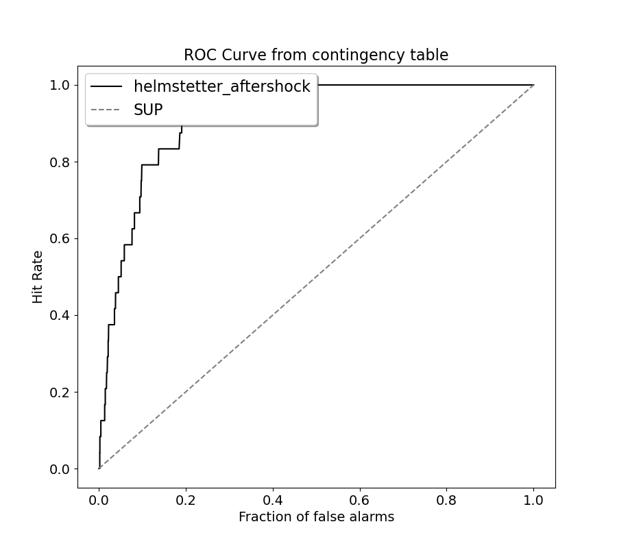
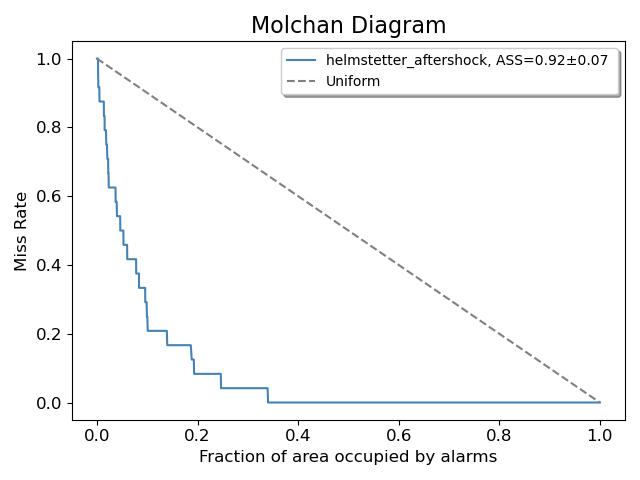
Plot ROC and Molchan curves using the alarm-based approach

#In this script, we generate ROC diagrams and Molchan diagrams using the alarm-based approach to evaluate the predictive
#performance of models. This method exploits contingency table analysis to evaluate the predictive capabilities of
#forecasting models. By analysing the contingency table data, we determine the ROC curve and Molchan trajectory and
#estimate the Area Skill Score to assess the accuracy and reliability of the prediction models. The generated graphs
#visually represent the prediction performance.

# Note: If "linear=True" the diagram is represented using a linear x-axis.
#       If "linear=False" the diagram is represented using a logarithmic x-axis.

print("Plotting ROC curve from the contingency table")
# Set linear True to obtain a linear x-axis, False to obtain a logical x-axis.
_ = plots.plot_ROC_diagram(forecast, catalog, linear=True)

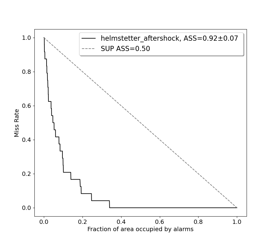
print("Plotting Molchan curve from the contingency table and the Area Skill Score")
# Set linear True to obtain a linear x-axis, False to obtain a logical x-axis.
_ = plots.plot_Molchan_diagram(forecast, catalog, linear=True)

• 
• 

Plotting ROC curve from the contingency table
Plotting Molchan curve from the contingency table and the Area Skill Score

Calculate Kagan’s I_1 score

We can also get the Kagan’s I_1 score for a gridded forecast (see Kagan, YanY. [2009] Testing long-term earthquake forecasts: likelihood methods and error diagrams, Geophys. J. Int., v.177, pages 532-542).

I_1 = get_Kagan_I1_score(forecast, catalog)
print("I_1score is: ", I_1)

I_1score is:  [2.31435371]