Working with catalog-based forecasts

This example shows some basic interactions with data-based forecasts. We will load in a forecast stored in the CSEP data format, and compute the expected rates on a 0.1° x 0.1° grid covering the state of California. We will plot the expected rates in the spatial cells.

Overview:

1. Define forecast properties (time horizon, spatial region, etc).

2. Compute the expected rates in space and magnitude bins

3. Plot expected rates in the spatial cells

Load required libraries

Most of the core functionality can be imported from the top-level csep package. Utilities are available from the csep.utils subpackage.

import numpy

import csep
from csep.core import regions
from csep.utils import datasets

Load data forecast

PyCSEP contains some basic forecasts that can be used to test of the functionality of the package. This forecast has already been filtered to the California RELM region.

forecast = csep.load_catalog_forecast(datasets.ucerf3_ascii_format_landers_fname)

Define spatial and magnitude regions

Before we can compute the bin-wise rates we need to define a spatial region and a set of magnitude bin edges. The magnitude bin edges # are the lower bound (inclusive) except for the last bin, which is treated as extending to infinity. We can bind these # to the forecast object. This can also be done by passing them as keyword arguments into csep.load_catalog_forecast().

# Magnitude bins properties
min_mw = 4.95
max_mw = 8.95
dmw = 0.1

# Create space and magnitude regions
magnitudes = regions.magnitude_bins(min_mw, max_mw, dmw)
region = regions.california_relm_region()

# Bind region information to the forecast (this will be used for binning of the catalogs)
forecast.region = regions.create_space_magnitude_region(region, magnitudes)

Compute spatial event counts

The csep.core.forecasts.CatalogForecast provides a method to compute the expected number of events in spatial cells. This requires a region with magnitude information.

_ = forecast.get_expected_rates(verbose=True)

Processed 1 catalogs in 0.001 seconds
Processed 2 catalogs in 0.002 seconds
Processed 3 catalogs in 0.003 seconds
Processed 4 catalogs in 0.003 seconds
Processed 5 catalogs in 0.004 seconds
Processed 6 catalogs in 0.005 seconds
Processed 7 catalogs in 0.005 seconds
Processed 8 catalogs in 0.006 seconds
Processed 9 catalogs in 0.007 seconds
Processed 10 catalogs in 0.008 seconds
Processed 20 catalogs in 0.014 seconds
Processed 30 catalogs in 0.021 seconds
Processed 40 catalogs in 0.028 seconds
Processed 50 catalogs in 0.035 seconds
Processed 60 catalogs in 0.042 seconds
Processed 70 catalogs in 0.048 seconds
Processed 80 catalogs in 0.055 seconds
Processed 90 catalogs in 0.062 seconds
Processed 100 catalogs in 0.068 seconds
Processed 200 catalogs in 0.131 seconds
Processed 300 catalogs in 0.197 seconds
Processed 400 catalogs in 0.262 seconds
Processed 500 catalogs in 0.355 seconds
Processed 600 catalogs in 0.420 seconds
Processed 700 catalogs in 0.485 seconds
Processed 800 catalogs in 0.581 seconds
Processed 900 catalogs in 0.645 seconds
Processed 1000 catalogs in 0.709 seconds
Processed 2000 catalogs in 1.491 seconds
Processed 3000 catalogs in 2.229 seconds
Processed 4000 catalogs in 2.987 seconds
Processed 5000 catalogs in 3.726 seconds
Processed 6000 catalogs in 4.466 seconds
Processed 7000 catalogs in 5.231 seconds
Processed 8000 catalogs in 5.940 seconds
Processed 9000 catalogs in 6.726 seconds
Processed 10000 catalogs in 7.388 seconds

Plot expected event counts

We can plot the expected event counts the same way that we plot a csep.core.forecasts.GriddedForecast

ax = forecast.expected_rates.plot(plot_args={'clim': [-3.5, 0]}, show=True)

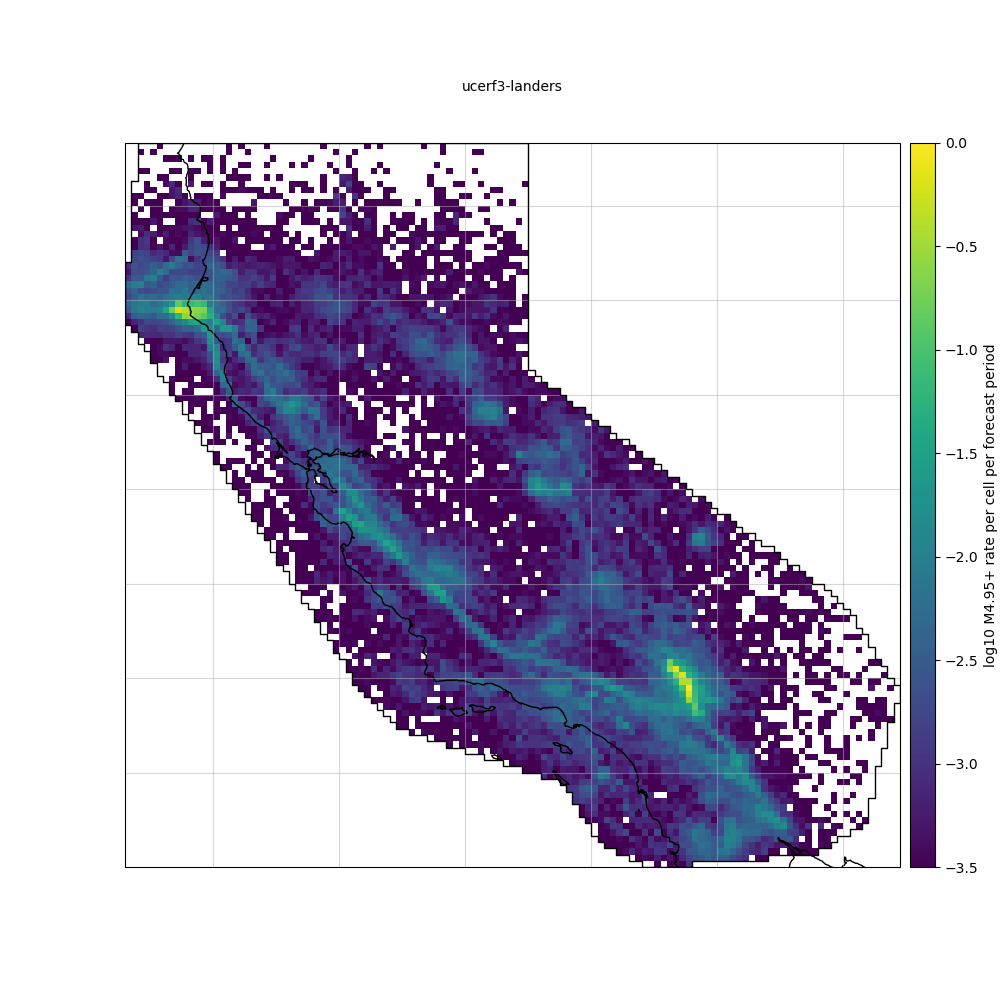
The images holes in the image are due to under-sampling from the forecast.

Quick sanity check

The forecasts were filtered to the spatial region so all events should be binned. We loop through each data in the forecast and count the number of events and compare that with the expected rates. The expected rate is an average in each space-magnitude bin, so we have to multiply this value by the number of catalogs in the forecast.

total_events = 0
for catalog in forecast:
    total_events += catalog.event_count
numpy.testing.assert_allclose(total_events, forecast.expected_rates.sum() * forecast.n_cat)